Blog
小さく始めて大きく育てるMLOps2020
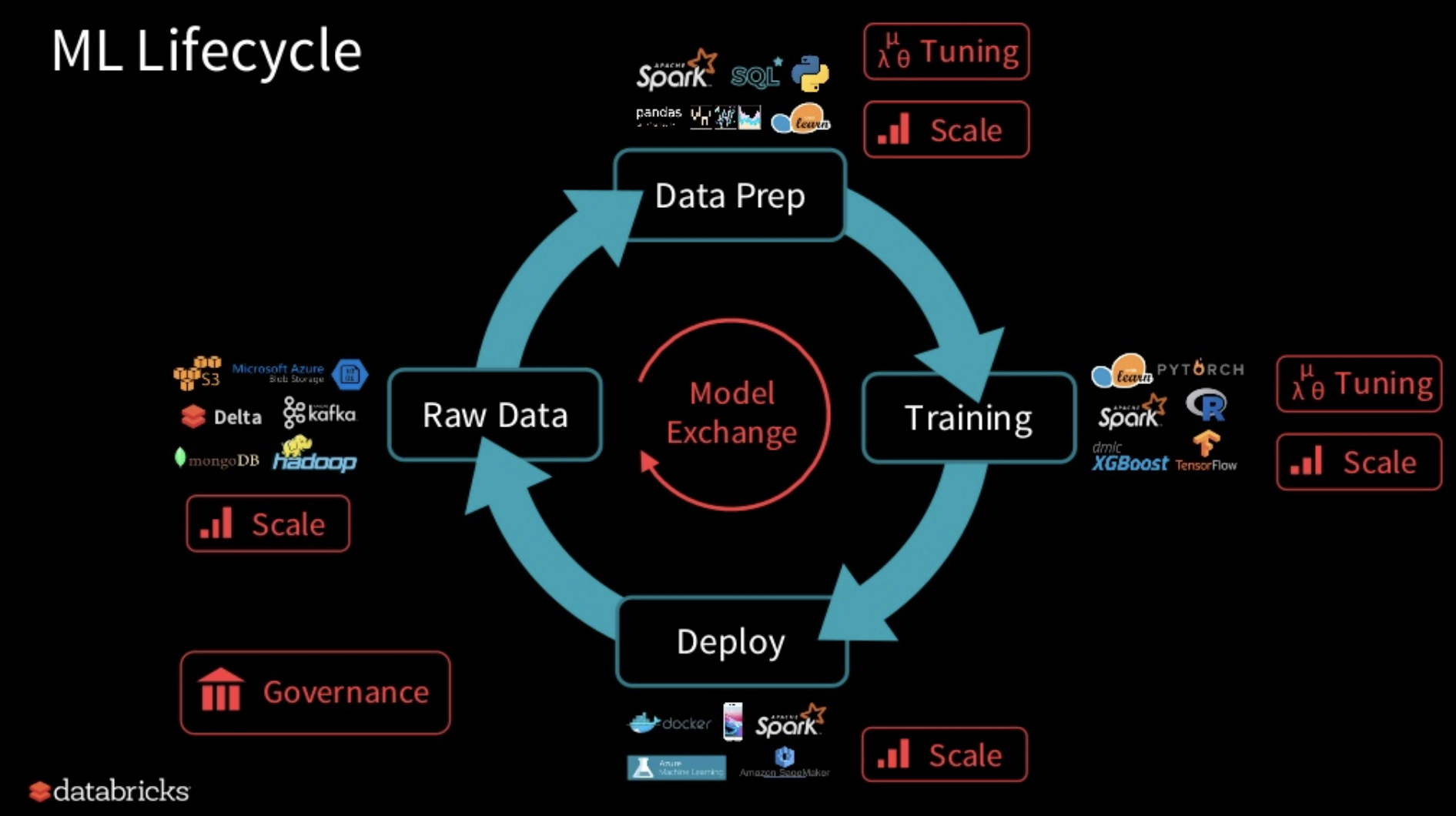
AI Labの岩崎(@chck)です、こんにちは。今日は実験管理、広義ではMLOpsの話をしたいと思います。
MLOpsはもともとDevOpsの派生として生まれた言葉ですが、本稿では本番運用を見据えた機械学習ライフサイクル(実験ログやワークフロー)の管理を指します。
参考記事のJan Teichmann氏の言葉を借りると、
エンジニアがDevOpsによって健全で継続的な開発・運用を実現している一方、
多くのデータサイエンティストは、ローカルでの作業と本番環境に大きなギャップを抱えている
- クラウド含む本番環境でのモデルのホスティングが考慮されないローカルでの作業
- 本番のデータボリュームやスケーリングを許容しないインメモリで少量のデータセットを使ったデータ処理
- 実験の再現性・冪等性のないJupyter Notebook
- 独立なタスクを組み合わせたETLパイプラインの構築(データの読込、モデルのトレーニングからスコアリングまで)がほとんどできていない
- ソフトウェアエンジニアリングのベストプラクティスがデータサイエンスプロジェクトに採用されにくい
- コードの抽象化、再利用性、単体テスト、ドキュメントやバージョン管理など
このような課題感から、機械学習ブームを引き連れた2020年現在において、Pythonや依存ライブラリの守備範囲は統計解析やモデリングの枠を超え(むしろここまではいい意味で枯れてきた)、システム実装のサポートや進歩したマシンリソースを携えた本番サーバーの上でどう運用していくかという段階まで広がりを見せています。
世はまさにMLOps時代、ツールの多さはRedditやMediumでも定期的に話題になる[1][2]ほどのレッドオーシャンで、各団体とも鎬を削って日々開発を行っています。しかし蓋を開けてみると、組み合わせて使うものや機能的に被るものが多く、結局どれ使ったらいいんじゃとなったので2020年現在の有力候補をサーベイしてみました。
tl;dr
下図の中から必要機能に応じて組み合わせましょう。
Hyperparametersはハイパーパラメータの管理や最適化機能を、Logging Experimentsは実験管理のための設定や結果の保存・可視化機能を、WorkflowはML Pipelineを実現できるツールをまとめています。
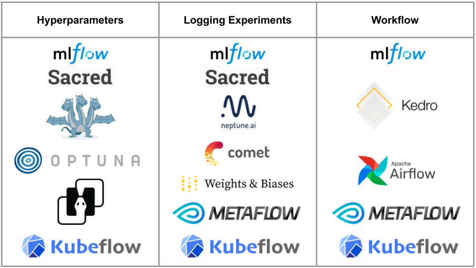
こうして見ると機能が広範囲なMLflow、Sacred、Metaflow、Kubeflowから選べば良さそうですが、ちょっと待ってください。高機能ほど往々にしてProjectへの導入ハードルが高いのです。
ブログタイトルの通り、まずは小さく始めましょう。おすすめはHydra、MLflow Tracking、Kedro、Optunaの組み合わせです。例えば次のようなユースケースが考えられます。
- Hydra + MLflow Tracking(Grid Search + Logging Experiments)
- MLflow Tracking + Kedro(Logging Experiments + Workflow)
- Optuna + MLflow Tracking + Kedro (Bayesian Search + Logging Experiments + Workflow)
MLflowにはParameter TuningからLogging Experiments、Workflowと一通りの機能が揃っていますが、Logging Experiments以外は高機能とは言えません。そこで、Workflow管理にKedroを、Parameter管理にHydraを組み合わせることで、より柔軟なMLOpsが始められるでしょう。密なJupyterLab連携やワークフロー管理がしたければKedro、ライブラリの依存を少なくしたいならMLflow単体という選択肢で、もちろん両刀もありです。ワンマンProjectであれば、無料版で事足りるNeptune.ai、Comet.ml、Weights & Biasesも選択肢に入りますが、メンバー間で実験の共有をしたくなったりすると有料版に踏み入ってしまうので最初から前述のセットがいいでしょう。また、実際には表のようにきれいに線引きできるほど分かれてはいないので、あくまでも目安にしてください。
そもそも馴染みのないツールもあると思いますので、ここからはそれぞれの特徴をさらっと解説していきます。コードスニペットや図も載せていくので、気になるツールの項だけでも参考になると幸いです。
Facebook Researchの開発するOSSの設定管理ツールです。Yaml間の設定値の継承・結合をしながらPython Objectとして読み込めるYaml Parserに、並列読込コマンドがおまけでついている感じです。ネストしたYamlの多重継承、変数の埋め込みなど、使用感はRuby製のYaml拡張であるLiquidに近いです。あくまで設定値の管理ツールなので、シンプルなConfig Parserとしても使うことができ、学習コストが低いのが魅力的。もちろん対象パラメータの組み合わせ探索として使えるので、Grid SearchのLauncherとして利用できます。
例えば以下のようなファイル構成を考えてみます。
|
1 2 3 4 5 6 |
. ├── config.yaml ├── model │ ├── catboost.yaml │ └── elastic_net.yaml ├── ex_hydra.py |
config.yamlというファイルを作り、”defaults”セクション内にネスト先のYamlの情報を加えます。
|
1 2 3 |
# config.yaml defaults: - model: elastic_net |
model ディレクトリ配下に今回はCatBoostとElasticNetのハイパーパラメータの初期値を書いておきます。config.yamlに従い、デフォルトではelastic_net.yamlが参照されます。
|
1 2 3 4 |
# model/catboost.yaml model: learning_rate: 0.05 depth: 10 |
|
1 2 3 4 5 |
# model/elastic_net.yaml model: alpha: 0.0005 l1_ratio: 0.9 random_state: 3 |
パラメータを読み込むMain関数を定義します。データセットやモデルの定義は省略していますが、受け取ったハイパーパラメータを使って学習する例です。
|
1 2 3 4 5 6 7 8 9 10 11 12 13 14 |
# ex_hydra.py import hydra from omegaconf import DictConfig @hydra.main(config_path="config.yaml") def my_ex(cfg: DictConfig) -> None: params = cfg.model print(params) model = get_model(params) model.fit(X, y) return r2_score(model.predict(X), y) if __name__ == "__main__": my_ex() |
ElasticNetのハイパーパラメータがYamlから読み込めています。
|
1 2 3 |
% python ex_hydra.py > {'alpha': 0.0005, 'l1_ratio': 0.9, 'random_state': 3} |
実行時引数で値を上書きできます。
|
1 2 3 |
% python ex_hydra.py model.l1_ratio=0.01 > {'alpha': 0.0005, 'l1_ratio': 0.01, 'random_state': 3} |
また、Multirun Optionによって予め定義しておいたパラメータを順番にセットしながら実行できたりします。便利。
|
1 2 3 4 5 6 7 8 |
% python ex_hydra.py -m model=elastic_net,catboost > [2020-05-20 13:15:45,284][HYDRA] Sweep output dir : multirun/2020-05-20/13-15-45 > [2020-05-20 13:15:45,285][HYDRA] Launching 2 jobs locally > [2020-05-20 13:15:45,285][HYDRA] #0 : model=elastic_net > {'alpha': 0.0005, 'l1_ratio': 0.9, 'random_state': 3} > [2020-05-20 13:15:45,374][HYDRA] #1 : model=catboost > {'learning_rate': 0.05, 'depth': 10} |
スイスの研究機関であるIDSIAの開発するOSSの実験管理ツールです。Hydraと違い実験管理に特化していて、実験ログの保存やUIを持ちます。Pythonデコレータベース(YamlやJSONも対応)で、pytest fixtureのような関数間のパラメータの共有(Injection) が特徴的。難点はMultirunの未対応[3]と、公式メンテのUIがないこと、デフォルトがMongoDB依存なことです。Logging Experimentsとしての機能を後述するNepture.aiなどのSaaSに移譲することで、MongoDB依存を切り捨てることもできます。
OmniboardというSacred用のWeb UIがありますが、MongoDBとNode依存が増えるので下記ではNeptune.aiと連携する例を紹介します。
|
1 2 3 4 5 6 7 8 9 10 11 12 13 14 15 16 17 18 19 20 21 22 23 24 25 26 27 28 29 30 31 32 33 34 35 36 |
# ex_sacred.py from sacred import Experiment from sacred.observers import FileStorageObserver from neptunecontrib.monitoring.sacred import NeptuneObserver import os ex = Experiment("elastic_net") # ex.observers.append(FileStorageObserver("sacredruns")) ex.observers.append(NeptuneObserver(api_token=os.environ["NEPTUNE_API_TOKEN"], project_name=os.environ["NEPTURE_PROJECT_NAME"])) @ex.config def parameters(): # Declare default parameters alpha = 0.0005 l1_ratio = 0.9 random_state = 3 @ex.capture def get_model(alpha: float, l1_ratio: float, random_state: int): from sklearn.linear_model import ElasticNet print("Parameters:", alpha, l1_ratio, random_state) return ElasticNet( alpha=alpha, l1_ratio=l1_ratio, random_state=random_state, ) @ex.main def run(): model = get_model() # Parameters are injected implicitly. model.fit(X, y) return r2_score(model.predict(X), y) if __name__ == "__main__": ex.run_commandline() |
SacredではObserverを設定することでログが書き込まれます。@ex.configでパラメータを定義し、@ex.captureや@ex.mainでパラメータを参照できます。
|
1 2 3 4 5 6 |
% python ex_sacred.py > INFO - elastic_net - Started > INFO - elastic_net - Result: 0.8940958224647267 > INFO - elastic_net - Completed after 0:00:02 > Parameters: 0.0005 0.9 3 |
Hydraのように、コマンドライン実行の場合はwith句で@ex.configのパラメータを上書きできますが、前述の通りMultirun未対応のため、Sacred Command自体をwrapする必要があります。
|
1 2 3 4 5 6 |
% python ex_sacred.py with 'l1_ratio=0.01' > INFO - elastic_net - Started > INFO - elastic_net - Result: 0.8940958224647267 > INFO - elastic_net - Completed after 0:00:02 > Parameters: 0.0005 0.01 3 |
Apache Sparkの祖であるMatei Zaharia氏が立ち上げたDatabricksの開発するOSSの実験管理用のツールです。今回紹介するツールの中でも機能の幅と学習コストのバランスが良く、MLflow Tracking, Projects, Modelsからなり、必要機能だけ切り出して使うことができます。公式サポートの実験管理UIを持ち、MLflow Trackingを通じて実験のログをS3やGCSに投げつつ、そのログを参照するMLflow Serverを立てておけば実験結果の共有も可能。
今回は目玉機能であるMLflow Trackingを中心に紹介します。キーワードとして、Parametersが入力パラメータ、Metricsが学習時のモデルのlossなど、Artifactsが画像やモデル、Python Pickleなどのバイナリデータの管理を司ります[4]。
まず、指定した場所に出力された実験のログファイルを参照、可視化できるMLflow Tracking Serverを立てておきます。
|
1 |
% mlflow server --backend-store-uri ./mlruns --default-artifact-root gs://YOUR_GCS_BUCKET/path/to/mlruns --host 0.0.0.0 |
–backend-store-uriにはMLflowが実験管理に使うメタデータの置き場所を指定します。I/Oの頻度が多いからか、SQLAlchemy互換のあるDBかlocal file systemしか選べません。Defaultは./mlrunsになります。–default-artifact-rootには前述したバイナリデータの置き場所を指定します。こちらはAWS, GCP, AzureのStorageやHDFSにも対応しています[5]。今回はメタデータはServerのlocalに、実験で使うバイナリデータはGCSにしてみます。Remote Serverで運用したい場合は、このように関連データのミドルウェアが一元化できないところが少し惜しいです。
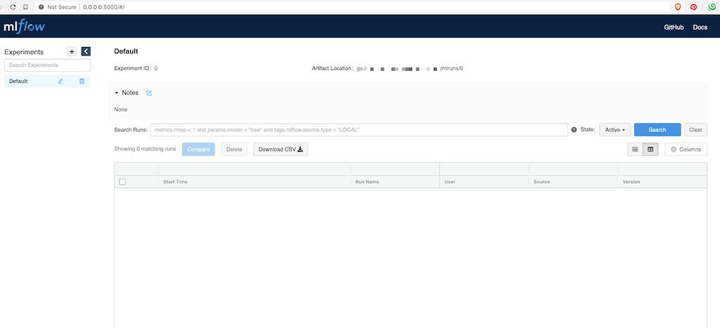
早速http://127.0.0.1:5000/にアクセスすると、MLflowの実験管理画面が確認できました。
Serverの準備ができたところで、実験ID(Name)の単位で実験を管理することができます。今回は実験名: MLMAN-1にParametersやMetrics、Artifactsを紐付ける形でモデルの学習をTrackingしてみましょう。
|
1 2 3 4 5 6 7 8 9 10 11 12 13 14 15 16 17 18 19 20 21 22 23 24 25 26 27 28 29 30 31 32 33 34 35 36 37 38 39 40 41 42 |
% mlflow_tracking.py import lightgbm as lgb from sklearn import datasets from sklearn.model_selection import train_test_split import mlflow import os iris = datasets.load_iris() X, y = iris.data, iris.target X_train, X_test, y_train, y_test = train_test_split(X, y, test_size=0.2, random_state=3) params = { "learning_rate": 0.05, "n_estimators": 500, } model = lgb.LGBMClassifier(**params) def mlflow_callback(): def callback(env): for name, loss_name, loss_value, _ in env.evaluation_result_list: mlflow.log_metric(key=loss_name, value=loss_value, step=env.iteration) return callback mlflow.set_tracking_uri(os.environ["MLFLOW_HOST"]) mlflow.set_experiment("MLMAN-1") with mlflow.start_run(): mlflow.log_params(params) model.fit( X_train, y_train, eval_set=(X_test, y_test), eval_metric=["softmax"], callbacks=[ lgb.early_stopping(10), mlflow_callback(), ]) # Log an artifact (output file) with open("output.txt", "w") as f: f.write("Hello world!") mlflow.log_artifact("output.txt") |
mlflow.set_tracking_uriには準備しておいたServerのhostを指定します。今回はhttp://127.0.0.1:5000になります。
|
1 2 3 |
% mlflow_tracking.py > INFO: 'MLMAN-1' does not exist. Creating a new experiment |
再度http://127.0.0.1:5000にアクセスすると、実験名: MLMAN-1で実験結果を確認できます。最高ですね。
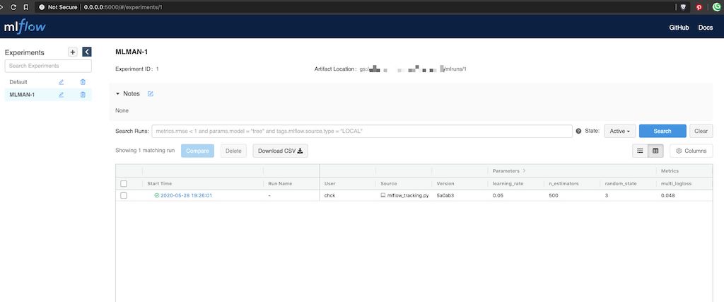
チームごとに1つ実験管理用のMLflow Tracking Serverを立てておいて、そこで実験結果の共有が行えると良いのではないでしょうか[6]。その他の機能において、ワークフロー管理やJupyterLab連携は後述するKedroに軍配が上がりそうですが、MLflow Trackingだけで機能十分とも言えます。
McKinsey & Companyの研究機関であるQuantum Black Labの開発するOSSのワークフロー管理ツールです。pandas.DataFrame化したデータの読込からモデリング・スコアリングまでの流れをPythonの関数として切り分けて定義しておき、自由に繋げてPipeline化できます。可視化機能付き[7]。キャッシュ化できるDataSetの管理に力を入れていて、SQL、File、S3などがビルトインで用意されている他、DataSet Classを継承してCustom DataSetも作成可能。また、JupyterLabとの連携が秀逸で、Pipeline側で定義したDataSetを参照できる他、JupyterLabのCell上で定義したFunctionをPipeline側に繋げることも。実験管理はサポートしていないのでMLflow Trackingなどと組み合わせるとBetter。ちょっとしたEDAはJupyterLabで行い、実際のワークフローはPipelineとして硬めに実装できます。
kedro newコマンドで以下のような雛形でProjectをScaffoldingしてくれます。
|
1 2 3 4 5 6 7 8 9 10 11 12 13 14 15 16 17 18 19 20 21 22 23 24 25 26 27 28 29 30 31 32 33 34 |
. ├── conf │ ├── base │ │ ├── catalog.yml │ │ ├── credentials.yml │ │ ├── logging.yml │ │ └── parameters.yml │ └── local ├── data │ ├── 01_raw │ │ └── iris.csv │ ├── 02_intermediate │ ├── 03_primary │ ├── 04_feature │ ├── 05_model_input │ ├── 06_models │ ├── 07_model_output │ └── 08_reporting ├── kedro_cli.py ├── notebooks └── src ├── tests │ ├── pipelines │ └── test_run.py └── tutorial ├── pipeline.py ├── pipelines │ ├── data_engineering │ │ ├── nodes.py │ │ └── pipeline.py │ └── data_science │ ├── nodes.py │ └── pipeline.py └── run.py |
ポイントはData Catalog、Parameter、NodeとPipelineです。ファイル数が多めですがそこまで複雑でないので順に見ていきましょう。
はじめにData Catalogです。Project内で共有したいDataをconf/base/catalog.ymlに定義していきます[8]。任意のデータ名をKeyに、データ形式をパースするためのコネクタ(実態はpythonで実装されたsave/loader)をtypeに指定し、filepathなどのコネクタに必要な引数を列挙します。
|
1 2 3 4 5 6 7 8 9 10 11 12 13 14 15 16 17 18 19 20 21 22 23 24 25 26 27 28 29 30 31 32 33 34 35 36 37 38 39 40 41 |
# conf/base/catalog.yml iris: type: pandas.CSVDataSet filepath: data/01_raw/iris.csv motorbikes: type: pandas.CSVDataSet filepath: s3://your_bucket/data/02_intermediate/company/motorbikes.csv credentials: dev_s3 load_args: sep: ',' skiprows: 5 skipfooter: 1 na_values: ['#NA', NA] scooters: type: pandas.SQLQueryDataSet credentials: scooters_credentials sql: > select * from cars where gear=4 load_args: index_col: [name] uscorn: type: api.APIDataSet url: https://quickstats.nass.usda.gov params: key: SOME_TOKEN format: JSON commodity_desc: CORN statisticcat_des: YIELD agg_level_desc: STATE year: 2000 example_model: type: pickle.PickleDataSet filepath: data/06_models/lightgbm.pkl.gz backend: joblib |
ここで定義されたDataがpandas.DataFrameやDictなどのPython ObjectとしてProject内のどこからでもsave/loadできるような仕組みになっています。ローカルのCSVはもちろん、S3上のファイルやSQL、API経由でのJSONなど、公式で十分すぎるほどのData Connectorが用意されている他、kedro.io.AbstractDataSetクラスを継承したオリジナルのData Connectorを作ることも出来るため、公式にない特殊なデータ形式を扱いたい場合でも、Pythonで処理を書けさえすればKedro Data Catalog機能の恩恵を受けながら自由に実装できます[9]。DataのVersioningにも対応しているのが嬉しいですね[10]。
dataディレクトリを見てみましょう。dataディレクトリは、前述したData Catalogで定義されたデータの実体が保管される場所で、loadが走る際にここにファイルがあるかの存在チェックによってデータのキャッシュ化を実現しています。特筆すべきはこのナンバリングされたディレクトリ構成です。データモデリングにおいて、生データの読込から、EDA、段階を踏んだ前処理の後、モデルの学習、モデル自体の保存、オフライン評価の結果の保存など、ワンサイクルだけでもデータが煩雑化してきます。Kedroでは、処理の段階に応じてデータを置き分けることを推奨しており、これによりデータの管理が健全になります。1-8は分かれ過ぎな気もしますが、公式からどの段階のデータはどこに置くべきかの指南書もあるので迷ったときは目を通すと良いでしょう[11]。
|
1 2 3 4 5 6 7 8 9 10 11 |
data ├── 01_raw │ └── iris.csv ├── 02_intermediate ├── 03_primary ├── 04_feature ├── 05_model_input ├── 06_models │ └── lightgbm.pkl.gz ├── 07_model_output └── 08_reporting |
全体的にシンプルに扱えるように上手に隠蔽されている一方、足りない部分はユーザが自由にカスタマイズできるような実装になっていて、非常に好感が持てました。
続いてParameterです。これも至ってシンプルで、Data CatalogがProject内で共有したいデータオブジェクトである一方、Parameterはその名の通りProject内で共有したいパラメータを定義できます。HydraやSacredのパラメータ管理機能親しく、parameters.ymlでintやstring・list型の値を管理し、後述するNode・Pipelineで参照することができます。
|
1 2 3 4 5 6 7 |
# conf/base/parameters.yml test_data_ratio: 0.2 epochs: 500 model: name: "lightgbm" learning_rate: 0.05 feature_fraction: 0.9 |
envで読み込むYamlを切り替えたり、ConfigLoaderをカスタマイズすることでHydraのような使用感に近づけることもできます[12]。そしてNodeとPipelineの説明です。ソースで言うところの以下の部分になります。
|
1 2 3 4 5 6 7 8 9 10 |
src └── tutorial ├── pipelines │ ├── data_engineering │ │ ├── nodes.py │ │ └── pipeline.py │ └── data_science │ ├── nodes.py │ └── pipeline.py └── run.py |
NodeはPipelineを組み立てる処理の一単位、PipelineはDataやParameterが共有されたNodeのチェーンを表します。まずdata_engineering/nodes.pyにiris dataに対する前処理、preprocess関数とsplit_data関数を定義します。
|
1 2 3 4 5 6 7 8 9 10 11 12 13 14 15 16 17 18 19 20 21 22 23 24 25 26 27 28 29 30 31 32 33 34 35 36 37 38 39 |
# pipelines/data_engineering/nodes.py from typing import Any, Dict, List import numpy as np import pandas as pd from sklearn.ensemble import IsolationForest from sklearn.model_selection import train_test_split from sklearn.preprocessing import MinMaxScaler def preprocess(iris: pd.DataFrame, random_state: int) -> List[Any]: X = iris[["sepal_length", "sepal_width", "petal_length", "petal_width"]] y = iris["species"] # Cut outliers clf = IsolationForest(max_samples=len(iris), random_state=random_state) clf.fit(X) y_noano = clf.predict(X) X = X.iloc[np.where(y_noano == 1)].reset_index(drop=True) y = y.iloc[np.where(y_noano == 1)].reset_index(drop=True) print("Number of Outliers:", len(np.where(y_noano == -1)[0])) print("Number of rows without outliers:", X.shape[0]) # Scaling mms_x = MinMaxScaler() X = pd.DataFrame(mms_x.fit_transform(X), columns=X.columns) return [X, y] def split_data(X: pd.DataFrame, y: pd.DataFrame, params: Dict[str, Any]) -> Dict[str, Any]: X_train, X_test, y_train, y_test = train_test_split(X, y, test_size=params["test_size"], random_state=params["random_state"]) return dict( X_train=X_train, y_train=y_train, X_test=X_test, y_test=y_test, ) |
data_engineering/pipeline.pyで前述した前処理関数をkedro.pipeline.nodeでwrapし、inputs・outputsで処理を繋ぐことでPipelineが出来上がりです。inputs・outputsには前述したcatalog.yml、parameters.ymlを参照することができ、指定した形式でload/saveされることで、Node間でDataやParametersを共有できます。Pipeline実行中だけに参照したい場合は、catalog.ymlの定義を省くことで内部でMemoryDataSetとして認識され、インメモリなオブジェクトとして扱うことも出来ます。
|
1 2 3 4 5 6 7 8 9 10 11 12 13 14 15 16 17 18 19 20 21 22 23 24 |
# pipelines/data_engineering/pipeline.py from kedro.pipeline import Pipeline, node from .nodes import preprocess, split_data def create_pipeline(**kwargs): return Pipeline( [ node( func=preprocess, inputs=["iris", "params:random_state"], outputs=["example_x", "example_y"], ), node( func=split_data, inputs=["example_x", "example_y", "parameters"], outputs=dict( X_train="example_train_x", y_train="example_train_y", X_test="example_test_x", y_test="example_test_y", ), ) ] ) |
前処理パイプラインが準備できたところで、学習パイプラインも同じように定義してみましょう。
|
1 2 3 4 5 6 7 8 9 10 11 12 13 14 15 16 17 18 19 20 21 22 23 24 25 26 27 28 29 30 31 32 33 34 35 36 |
# pipelines/data_science/nodes.py import logging from typing import Any, Dict import lightgbm as lgb import pandas as pd from sklearn.metrics import accuracy_score def train_model( X_train: pd.DataFrame, y_train: pd.DataFrame, X_test: pd.DataFrame, y_test: pd.DataFrame, parameters: Dict[str, Any] ) -> Any: if parameters["model"]["name"] == "lightgbm": params = { "learning_rate": parameters["model"]["learning_rate"], "n_estimators": parameters["epochs"], } model = lgb.LGBMClassifier(**params) model.fit( X_train, y_train, eval_set=(X_test, y_test), eval_metric=["softmax"], callbacks=[lgb.early_stopping(10)], ) else: raise NotImplementedError return model def report_accuracy(model: Any, X_test: pd.DataFrame, y_test: pd.DataFrame) -> None: accuracy = accuracy_score(y_test, model.predict(X_test)) log = logging.getLogger(__name__) log.info("Model accuracy on test set: %0.2f%%", accuracy * 100) |
|
1 2 3 4 5 6 7 8 9 10 11 12 13 14 15 |
# pipelines/data_science/pipeline.py from kedro.pipeline import Pipeline, node from .nodes import report_accuracy, train_model def create_pipeline(**kwargs): return Pipeline( [ node( func=train_model, inputs=["example_train_x", "example_train_y", "example_test_x", "example_test_y", "parameters"], outputs="example_model", ), node(func=report_accuracy, inputs=["example_model", "example_test_x", "example_test_y"], outputs=None), ] ) |
ディレクトリがdata_engineeringとdata_scienceに分かれていますが、dataでいう01_raw – 04_featureまでのデータの前処理までをdata_engineeringに、05_model_input 以降をdata_scienceにまとめると見通しが良くなります。
Pipelineが一通り定義できたら、最後にPipelinesの実行順を担うマッピングを定義します。
|
1 2 3 4 5 6 7 8 9 10 11 12 13 14 15 |
# tutorial/pipeline.py from typing import Dict from kedro.pipeline import Pipeline from tutorial.pipelines import data_engineering as de from tutorial.pipelines import data_science as ds def create_pipelines(**kwargs) -> Dict[str, Pipeline]: data_engineering_pipeline = de.create_pipeline() data_science_pipeline = ds.create_pipeline() return { "de": data_engineering_pipeline, "ds": data_science_pipeline, "__default__": data_engineering_pipeline + data_science_pipeline, } |
これで準備が整いました。Kedroパイプラインを実行してみましょう。
|
1 2 3 4 5 6 7 8 9 10 11 12 13 14 15 16 17 18 19 20 21 22 23 24 25 26 27 28 29 30 31 32 |
% kedro run > INFO - Loading data from `iris` (CSVDataSet)... > INFO - Loading data from `params:random_state` (MemoryDataSet)... > INFO - Running node: preprocess([iris,params:random_state]) -> [example_x,example_y] > INFO - Saving data to `example_x` (MemoryDataSet)... > INFO - Saving data to `example_y` (MemoryDataSet)... > INFO - Completed 1 out of 4 tasks > INFO - Loading data from `example_x` (MemoryDataSet)... > INFO - Loading data from `example_y` (MemoryDataSet)... > INFO - Loading data from `parameters` (MemoryDataSet)... > INFO - Running node: split_data([example_x,example_y,parameters]) -> [example_test_x,example_test_y,example_train_x,example_train_y] > INFO - Saving data to `example_train_x` (MemoryDataSet)... > INFO - Saving data to `example_train_y` (MemoryDataSet)... > INFO - Saving data to `example_test_x` (MemoryDataSet)... > INFO - Saving data to `example_test_y` (MemoryDataSet)... > INFO - Completed 2 out of 4 tasks > INFO - Loading data from `example_train_x` (MemoryDataSet)... > INFO - Loading data from `example_train_y` (MemoryDataSet)... > INFO - Loading data from `example_test_x` (MemoryDataSet)... > INFO - Loading data from `example_test_y` (MemoryDataSet)... > INFO - Loading data from `parameters` (MemoryDataSet)... > INFO - Running node: train_model([example_test_x,example_test_y,example_train_x,example_train_y,parameters]) -> [example_model] > INFO - Saving data to `example_model` (MemoryDataSet)... > INFO - Completed 3 out of 4 tasks > INFO - Loading data from `example_model` (MemoryDataSet)... > INFO - Loading data from `example_test_x` (MemoryDataSet)... > INFO - Loading data from `example_test_y` (MemoryDataSet)... > INFO - Running node: report_accuracy([example_model,example_test_x,example_test_y]) -> None > INFO - Model accuracy on test set: 91.30% > INFO - Completed 4 out of 4 tasks > INFO - Pipeline execution completed successfully. |
catalog.yml, parameters.ymlを参照しながら、nodeに定義した関数が inputs -> func -> outputs -> inputs -> func…と数珠繋ぎに実行されている様子がわかりますね。
kedro runに–pipelineオプションを渡すことで特定のパイプラインを実行することもできますが、今回のようにdata_engineeringパイプラインのoutputsをMemoryDataSetとしている(catalog.ymlに書いていない)場合は、data_scienceパイプラインだけを実行してもdata_engineeringのoutputsは参照できないので注意しましょう。
|
1 2 3 |
% kedro run --pipeline ds > ValueError: Pipeline input(s) {'example_train_x', 'example_test_y', 'example_test_x', 'example_train_y'} not found in the DataCatalog |
小さく動かすためにはここまで抑えておけば十分です。Pipelineを構成する要素として紹介したNodeやData、ParameterはKedro Project内で共有できるため、notebooksディレクトリのJupyterLabからも参照できます。更に、JupyterLabのtag機能を応用してcell上で定義した関数をnode化したり[13]、JupyterLab上でPipelineの実行も可能なため、インタラクティブに分析しつつ、FunctionalなData Pipelineを構築することができます。具体的にはnodes.pyに関数をまとめて定義しておき、JupyterLabからは参照メインにすることで、共通化したい関数が散らばることなく健全です。また、Kedro単体ではParameter Tuningや実験管理機能を持たないので、Data Catalogから読み込んだconfig.ymlやparameters.ymlをOptunaと連携させつつMLflow Trackingで実験管理すると良いでしょう[14]。後述するApache Airflowにも対応しているためCloud Service (Cloud Composer/AWS Airflow)と連携したWorkflow管理も可能です。
Neptune.ai, Comet.ml, Weights & Biases
それぞれMLスタートアップの提供するSaaSの実験管理ツールで、Python APIを通じて実験ログをSaaSに流し、Web UI上で実験の可視化や共有ができます。機能差はそこまで無いです。個人利用は無料、チーム利用やストレージ上限開放が定額制なパターンが多く、SaaSなのでユーザ側でインフラの準備が要らないのが特徴。
Neptune.aiの例を紹介します。使用感はMLflow Trackingに近いです。Neptune側でMonitoringするcallback関数を渡す他、インテグレーションが豊富に実装されているので、機械学習ライブラリと簡単に連携できます。
|
1 2 3 4 5 6 7 8 9 10 11 12 13 14 15 16 17 18 19 20 21 22 23 24 25 26 27 28 29 30 31 32 33 34 35 |
import neptune import lightgbm as lgb import os params = { 'boosting_type': 'gbdt', 'num_leaves': 31, 'learning_rate': 0.05, 'feature_fraction': 0.9, 'n_estimators': 500, } neptune.init(os.environ["NEPTURE_PROJECT_NAME"]) neptune.create_experiment(name="lightgbm", params=params) def neptune_callback(): def callback(env): for name, loss_name, loss_value, _ in env.evaluation_result_list: neptune.send_metric('{}_{}'.format(name, loss_name), x=env.iteration, y=loss_value) return callback model = lgb.LGBMRegressor(**params) model.fit( X_train, y_train, eval_set=(X_test, y_test), eval_metric=["mae", "mse"], callbacks=[ lgb.early_stopping(10), neptune_callback(), ] ) neptune.stop() |

実験に使ったパラメータと結果が管理画面から確認できる
Netflixの開発するOSSのワークフロー管理ツールです。@stepデコレータを繋げていくことでWorkflowを定義します。実験管理とワークフロー機能を持ちますが、実験の可視化UIを持たず、ログが管理できるだけなので今後に期待。Documentを見る感じ、AWS連携に力を入れているようです[15]。
|
1 2 3 4 5 6 7 8 9 10 11 12 13 14 15 16 17 18 19 20 21 22 23 24 25 26 27 28 29 30 |
from metaflow import FlowSpec, step class SampleFlow(FlowSpec): @step def start(self): """ This is the 'start' step. All flows must have a step named 'start' that is the first step in the flow. """ print("SampleFlow is starting.") self.next(self.hello) @step def hello(self): """ This is a middle step. """ print("Metaflow says: Hi!") self.next(self.end) @step def end(self): """ This is the 'end' step. All flows must have an 'end' step, which is the last step in the flow. """ print("SampleFlow is all done.") if __name__ == '__main__': SampleFlow() |
Googleの開発するOSSの機械学習プラットフォームです。図の通りハイパーパラメータ最適化からワークフローまでカバーしており高機能ですが、Kubernetes上での稼働前提なのと依存ライブラリが多いので学習コストは重め。もともとTensorFlowのMLOps拡張として作られていた背景柄、GCPやTensorFlowと相性が良いので、GCPをメインに据える場合は特に強い武器になるでしょう。

https://www.kubeflow.org/docs/started/kubeflow-overview/
Airbnb発のOSSのワークフローエンジンです。Hydraと同じくMLに特化したツールではないですが、ワークフロー系のツールのコアとなるので合わせて紹介させてください。Pure PythonでPipelineを記述でき、UIによるワークフローの可視化、スケジューリング機能などを持ちます。AWS, GCPを始めとする様々なサービスでサポートされていて[16]、MLflowやKedroとも連携ができるので、これらツールをクラウド化する際の橋渡しになるでしょう。
|
1 2 3 4 5 6 7 8 9 10 11 12 13 14 15 16 17 18 19 20 21 22 23 24 25 26 27 28 29 30 31 32 33 |
from airflow import DAG from airflow.operators.bash_operator import BashOperator from datetime import datetime dag = DAG( dag_id="sample_pipeline", default_args={ "start_date": datetime.now() }, ) task1 = BashOperator( task_id="print_date", bash_command="date", dag=dag, ) task2 = BashOperator( task_id="echo_a", depends_on_past=False, bash_command="echo 'a'", dag=dag, ) task3 = BashOperator( task_id="echo_b", depends_on_past=False, bash_command="echo 'b", dag=dag, ) # A list of tasks can also be set as dependencies. task1 >> [task2, task3] |
Scikit-LearnよろしくOSSのハイパーパラメータ最適化フレームワークです。局所解に陥りにくいガウス過程を元にしたベイズ最適化が実装されていますが、適切な設定値が与えられていないと非効率な探索となり計算量が増大する[17]という欠点があります。
|
1 2 3 4 5 6 7 8 9 10 11 12 13 14 |
%%time from skopt.space import Integer def objective(x): return (x[0] - 2) ** 2 space = [ Integer(-10, 10, name="x") ] result = gp_minimize(objective, space) result.x |
|
1 2 |
Wall time: 1min 11s [2] |
Preferred Networksの開発するOSSのハイパーパラメータ最適化フレームワークです。前述したskoptの欠点を克服したTPE[18]というアルゴリズムを採用している他、IntegrationとしてOptuna APIからskopt等を呼び出して利用することもできます。
|
1 2 3 4 5 6 7 8 9 10 11 12 |
%%time import optuna def objective(trial): x = trial.suggest_uniform("x", -10, 10) return (x - 2) ** 2 study = optuna.create_study() study.optimize(objective, n_trials=100) study.best_params |
|
1 2 |
Wall time: 4.58 s {'x': 1.996326922833609} |
まとめ
2020年有力であろうMLOpsのためのツールをかいつまんで紹介しました。今回紹介した機能はほんの一部ですので、今後のロードマップなどの詳細は各公式サイトを参照ください。これからはじめるよという方は、まずは小さく導入してみて、皆さんのProjectの状況やツールの馴染み具合に従って高機能な組み合わせやAll-in-oneなツール(x-flow系)、Managedなツール(AI Platform 、SageMaker等)に移っていくと良いでしょう。MLOpsや実験管理を意識したProjectを進める上で重要なのは、「どのパラメーターで実験して結果がどうなったか」「実装コードの書き捨てが引き継ぎや再現のコストになっていないか」「ツールにどこまで求めるか」を把握できているかです。今回紹介した何かしらのツールの思想に乗っかることでオレオレプロジェクトに秩序が生まれ、再利用性の高い実験コードに変わります。ワンマンプロジェクトでも数十人のプロダクトでも、使えるツールは使ってみんなが幸せになればいいのです。
刹那的なコードではなく、使い回しを意識した実験管理を今日からはじめましょう。
ソースコード: https://github.com/chck/ml-management-tools
参考文献
Complete Data Science Project Template with Mlflow for Non-Dummies
How do you manage your Machine Learning Experiments?
ML Best Practices: Test Driven Development at Latent Space
- https://www.reddit.com/r/MachineLearning/comments/bx0apm/d_how_do_you_manage_your_machine_learning/ ↩
- https://www.kdnuggets.com/2020/01/managing-machine-learning-cycles.html ↩
- https://github.com/IDSIA/sacred/issues/727#issuecomment-610798059 ↩
- https://www.mlflow.org/docs/latest/tracking.html#concepts ↩
- https://www.mlflow.org/docs/latest/tracking.html#artifact-stores ↩
- ただし、HTTPS化や認証をかけたい場合はnginxを挟むなど別途工夫が必要になります。 ↩
- https://github.com/quantumblacklabs/kedro-viz ↩
- https://kedro.readthedocs.io/en/stable/04_user_guide/04_data_catalog.html ↩
- https://kedro.readthedocs.io/en/stable/04_user_guide/08_advanced_io.html ↩
- https://kedro.readthedocs.io/en/latest/04_user_guide/04_data_catalog.html#versioning-datasets-and-ml-models ↩
- https://kedro.readthedocs.io/en/latest/06_resources/01_faq.html#what-is-data-engineering-convention ↩
- https://kedro.readthedocs.io/en/latest/04_user_guide/03_configuration.html#additional-configuration-environments ↩
- https://kedro.readthedocs.io/en/stable/04_user_guide/11_ipython.html#converting-functions-from-jupyter-notebooks-into-kedro-nodes ↩
- https://medium.com/@QuantumBlack/deploying-and-versioning-data-pipelines-at-scale-942b1d81b5f5 ↩
- https://docs.metaflow.org/metaflow-on-aws/metaflow-on-aws ↩
- https://airflow.apache.org/docs/stable/installation.html#extra-packages ↩
- https://tech.preferred.jp/ja/blog/limited-gp/ ↩
- https://papers.nips.cc/paper/4443-algorithms-for-hyper-parameter-optimization.pdf ↩
Author